Objective

This blog is inspired from the wildml blog on text classification using convolution neural networks. This blog is based on the tensorflow code given in wildml blog. Here, in this blog i have taken two senetences as example and tried to explain what happens to the input data at each layer of the CNN. For each layer of the network it explains input for the layer, processing done and the output of each layer along with the shape of input and output data.
This blog does not explains the basic working of CNN. It assumes that the reader has some understanding of CNN’s

Github link to the code being explained.

I will try to explain the network in the same order as it is in code.

1. Data processing
2. Embedding Layer
3. Convolution Layer
4. Pooling Layer
5. Dropout Layer
6. Output Layer

I Will be using following two sentences as input for our classification task:

Sentence 1 : The camera quality is very good
Sentence 2 : The battery life is good

Here we have two sentences of length 6 and 5 respectively.
We also assume that their are two classes for our classification model, Positive and Negative.

Data preprocessing and building the vocabulary

Since the sentences are of different length, we pad our sentences with special <PAD> token to make the lengths of the two sentences equal.

So now we have our sentences modified as :
Sentence 1 : the camera quality is very good
Sentence 2 : the battery life is good <PAD>.
Now, both the sentences are of same length. We proceed to build the vocabulary index.
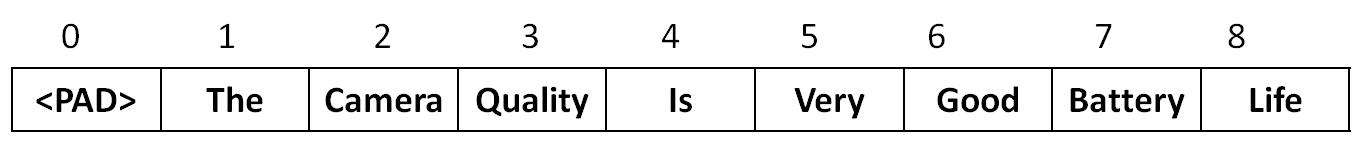
Vocabulary index is a mapping of integer to each unique word in the corpus.
In our case, size of vocabulary index will be 9, since there are 9 unique tokens. Vocabulary is as follows

Corresponding code from the blog

vocab_processor = learn.preprocessing.VocabularyProcessor(max_document_length)

In tensorflow, tensorflow.contrib.learn.preprocessing.VocabularyProcessor is used for building the vocabulary.
Use this link to see how to extract vocabulary from the vocab_processor object.

Next, each sentence is converted into vector of integers.
Sentence 1 : [1, 2, 3, 4, 5, 6]
Sentence 2 : [1, 7, 8, 4, 6, 0]

Embedding Layer

Configurable parameters for embedding layer

• batch_size = 2 (Since we have only two sentences here)
• sequence length = 6 (Max length of the senteces)
• num_classes = 2 (Number of output classes. Positive and negative in our case)
• vocabulary size (V) = 9

Trainable parameters for embedding layer

• Embedding vector size (E) = 128 (Size of the embedding vector)
• Embedding matrix (W) of shape = [V * E] = [9 * 128]

Input

• shape of input (input_x) = [batch_size, sequence_length] = [2, 6]
• shape of input (input_y) = [batch_size, num_classes] = [2, 2]
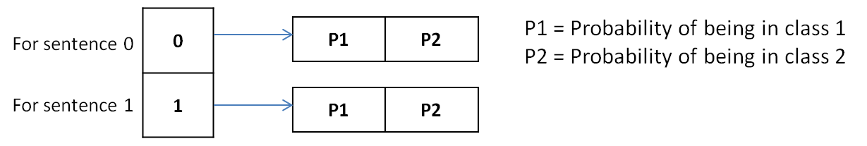
  Here, input_y are the output labels of input sentences encoded using one-hot encoding. Assuming both the sentences are positive (which will not be the actual case. There will also be negative sentences.)
  input_y = [ [1, 0], [1,0] ]

Working of embedding layer

As per the code in the wildml blog:

self.input_x = tf.placeholder(tf.int32, [None, sequence_length], name="input_x")

Input to the embedding layer is a tuple whose length is equal to the batch size, i.e, number of sentences in a batch.
Each element of the tuple is an array of numbers, representing sentence in the form of indexes into vocabulary.
For example :

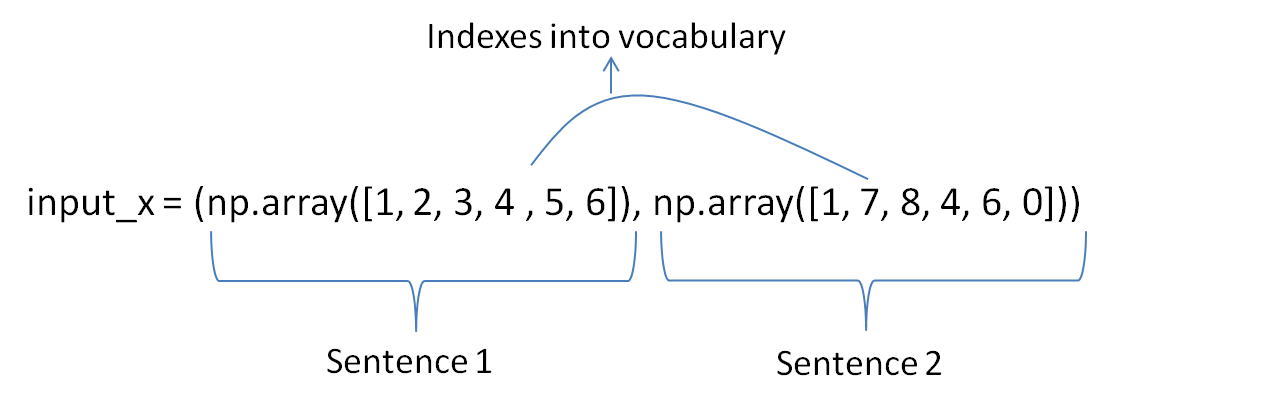
Embedding Lookup

Statement from the wildml blog

self.embedded_chars = tf.nn.embedding_lookup(w, self.input_x)

This statement takes as input, input_x from the previous step.
For each sentence, and for each word, it looks up (indexes) the embedding matrix (which is 9 * 128 in our case) (w) and returns the corresponding embedding vector for each word of each sentence.
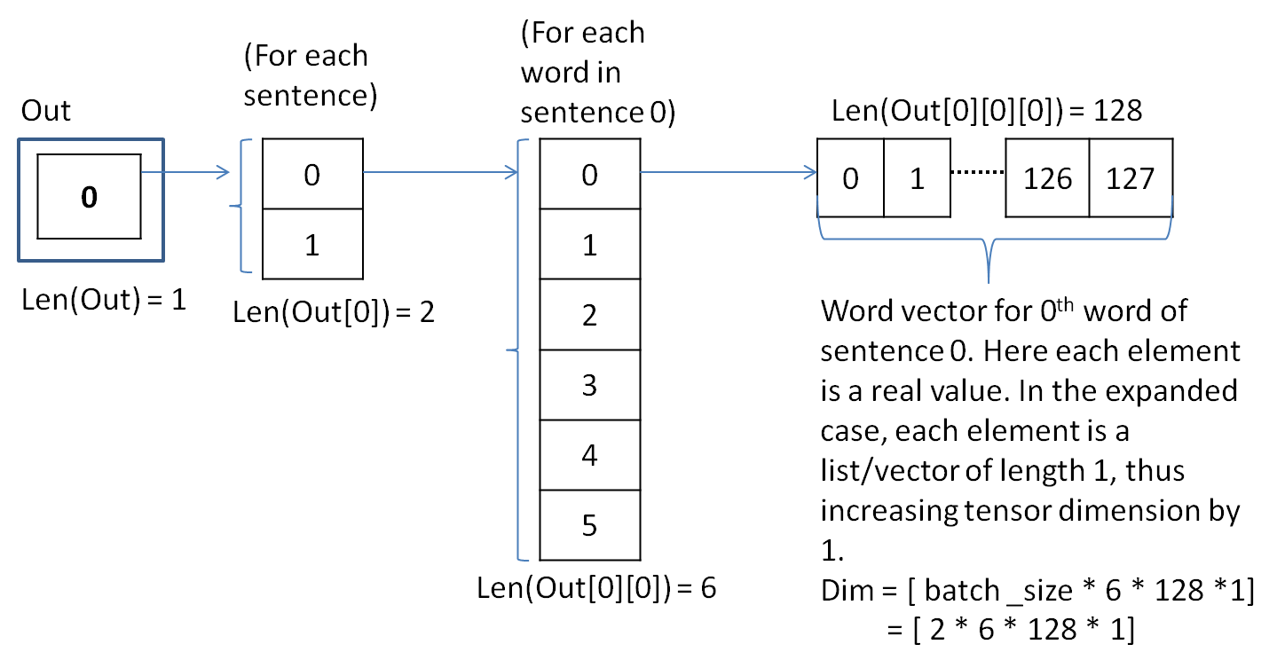
When i printed the variable embedded_chars, it is actually a list structured as follows :

• embedded_chars is a list of size 1,
• its 0th element is a list of size batch_size, i.e, number of sentences, (2 for this ex)
• each element of this list is a list of size sequence_length, (6 for this ex)
• and, each element of this list is a list of size embedding vector (128 for this ex.)

Here, the shape of tensor is [batch_size, sequence_length, embedding_vector_length], i.e, [2 * 6 * 128].

Each element of the word vector is a real value. In the next satement of the blog, i.e,

self.embedded_chars_expanded = tf.expand_dims(self.embedded_chars, -1)

tensor is reshaped to [batch_size, sequence_length, embedding_vector_length, 1],
i.e, [2 * 6 * 128 * 1]. So that, each element of the word vector is itself a list of size 1, instead of a real number.
Both the above statements can be easily understood from the following figure, where out = embedded_chars

This completes the explanation of embedding layer

Output of embedding layer :

• Tensor of shape : [batch_size, sequence_length, embedding_vector_length, 1], i.e, [2 * 6 * 128 * 1]. Next layer in the model is the convolution layer.

Convolution Layer

Configurable parameters of convolution layer

• filter_sizes : 3, 4, 5
• num_filters: 128
• Stride length : [1 * 1 * 1 * 1]
• Padding : VALID
  As oppossed to 2D filters in images, here in text classification we use 1D filters. We will be using filters of sizes 3,4,5. First we will go through the process of a single filter. Same will work for the other two sizes. Later we will see, how to merge the output from all the three filter sizes.

Trainable parameters of convolution layer

• Weight matrix (W) : its shape is same as shape of filter.(Discussed next)
• Bias(b) : = [0.1, 0.1, 0.1……..0.1] Since there are 128 filters, there will be 128 bias values.

Input

• Output of the expanded embedding lookup step. Its shape is
  [batch_size, sequence_length, embedding_vector_length, 1], i.e, [2 * 6 * 128 * 1]

Now, what is the shape of filter ? Lets take filter of size, filter_size = 3. In this case, shape of the filter is [filter_height, fiter_width] or [filter_size, embedding_vector_length] or [3 * 128]. This means that the filter sees 3 words (or embedding vectors) at a time, and based on the stride keeps seeing the 3 word vectors.
We have only one input channel, therefore, num_input_channels = 1
Number of output channels or Number of filters is 128. Therefore, shape of the filter tensor becomes : [filter_size, embedding_vector_len, num_input_channels, num_filters] = [ 3 * 128 * 1 * 128] The following figure shows the mapping between input matrix and filter of size 3 :
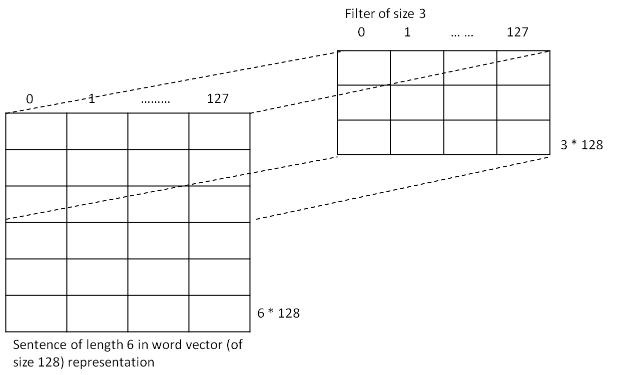
Here, the input only represents one sentence NOT both.
I will explain how to apply convolution filter on the input in the next step, but, before that let us see how to compute the output shape for this filter of size 3.

Now, what is the shape of output filter ?
For 1D case, as in text,
out_rows = (W1- F + 2 * P) / S + 1
where,
W1 = sequence_length (Number of input words) = 6 (in our case)
F = height of filter or filter size = 3 (in our case)
P = padding = 0 (in our case)
Stride = 1 (in our case)

Therefore,
out_rows = (6 - 3 + 2 * 0) / 1 + 1 = 4
Since the filter moves only in 1D, shape of output = 4 * 1, for a single sentence with a fiter_size = 3 and for one output channel.
Now, since we have batch of sentences and num_filters = 128, we get 4 * 1 outputs for each combination. Therefore, shape of output tensor for fiter_size (3) is
[batch_size * 4 * 1 * num_filters] = [2 * 4 * 1 * 128]

Similarly, we can compute the output shapes for filters of size 4 and 5 as follows :
For filter_size (4) (6 - 4 + 2 * 0) / 1 + 1 = 3 or [2 * 3 * 1 * 128]
For filter_size (5) (6 - 5 + 2 * 0) / 1 + 1 = 2 or [2 * 2 * 1 * 128]
Now let us see a simple calculation showing how filter is applied to input and what is the role of weight matrix and bias.
Corresponding code statement:

conv = tf.nn.conv2d(self.embedded_chars_expanded, W,
                    strides=[1, 1, 1, 1],
                    padding="VALID",
                    name="conv")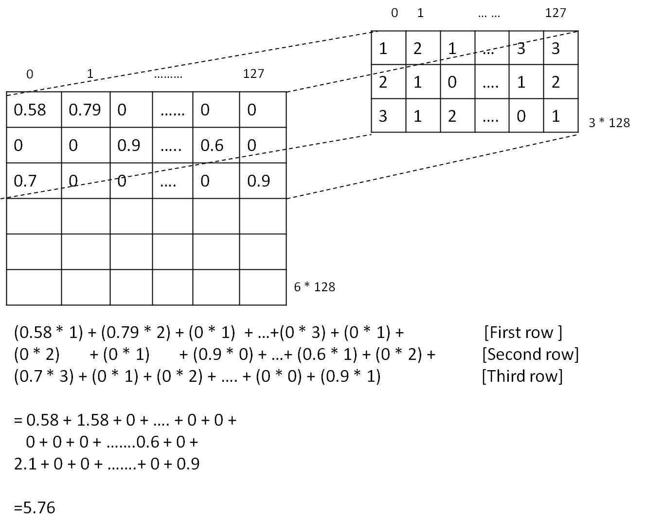

From the above figure, we get the result of applying fiter to patch of size 3 * 128, which is 5.76.
In the case of tensorflow conv2d function, the conv2d function only performs elementwise multiplication of input patch and filter. The bias needs to be added separately.
This is done in the next line of the code where nonlinearity is being applied along with bias addition.

h = tf.nn.relu(tf.nn.bias_add(conv, b), name="relu")

Here, bias is being added to the output of conv layer for each patch-filter convolution. So, for the current patch we get 5.76 + 0.1 = 5.86. On this output, relu is applied to, i.e, max(0, x) = max(0, 5.86) = 5.86 So, we get h = 5.86 for the current patch. The figure below describes the process for all the filters i.e, num_filters = 128.

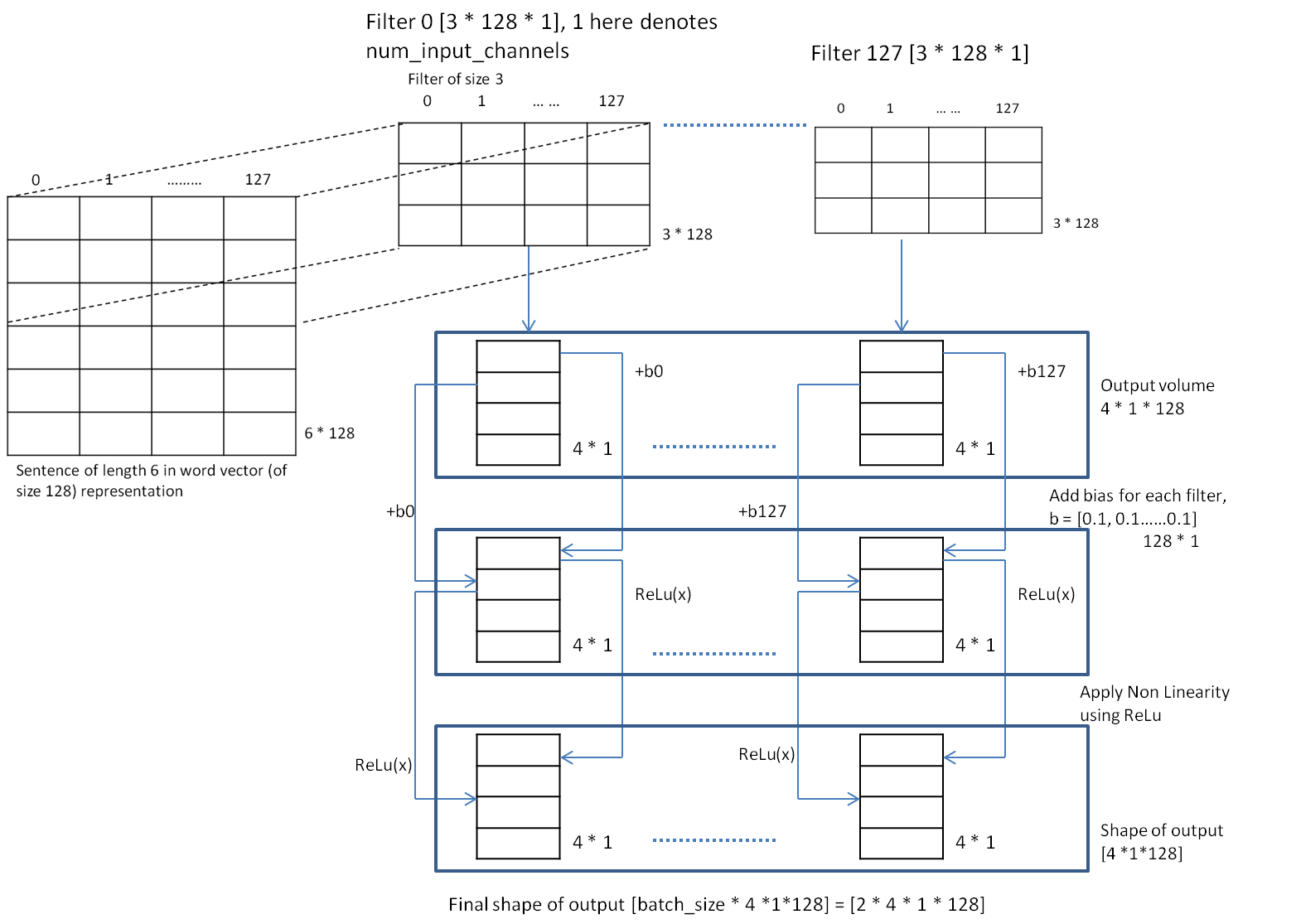
The figure above shows the output, for, when 128 filters of size 3 are applied on a single sentence. When applied to batch, shape becomes [batch_size * 4 * 1 * 128] = [2 * 4 * 1 * 128]

Pooling Layer

Configurable parameters of pooling layer

• ksize : shape of the pool operator [1 * 4 * 1 * 128]
• strides : same as conv2d [1 * 1 * 1 * 1]

Their are no training parameters for this layer. As only max operation is performed.
Corresponding code statement:

pooled = tf.nn.max_pool(h, ksize=[1, sequence_length - filter_size + 1, 1, 1],
                    strides=[1, 1, 1, 1],
                    padding='VALID',
                    name="pool")

Input

Output of the convolution layer, whose shape is [batch_size * 4 * 1 * num_filters ] = [2 * 4 * 1 * 128]. Here, we are using the output from the filter of size, filter_size = 3
In the max pooling layer we perform max operation on the output of each filter over the sentence, i.e, max operation on the 4 * 1 output of each filter. The max can be selected from all the 4 values, or we can define a different ksize.
Here, we are using ksize = [1 * (4 * 1) * 128], which means select the max out of all the four values. Since the selection is done from all the values, we get a single value as output for each of the 128 filters. This is demonstrated in the figure below :

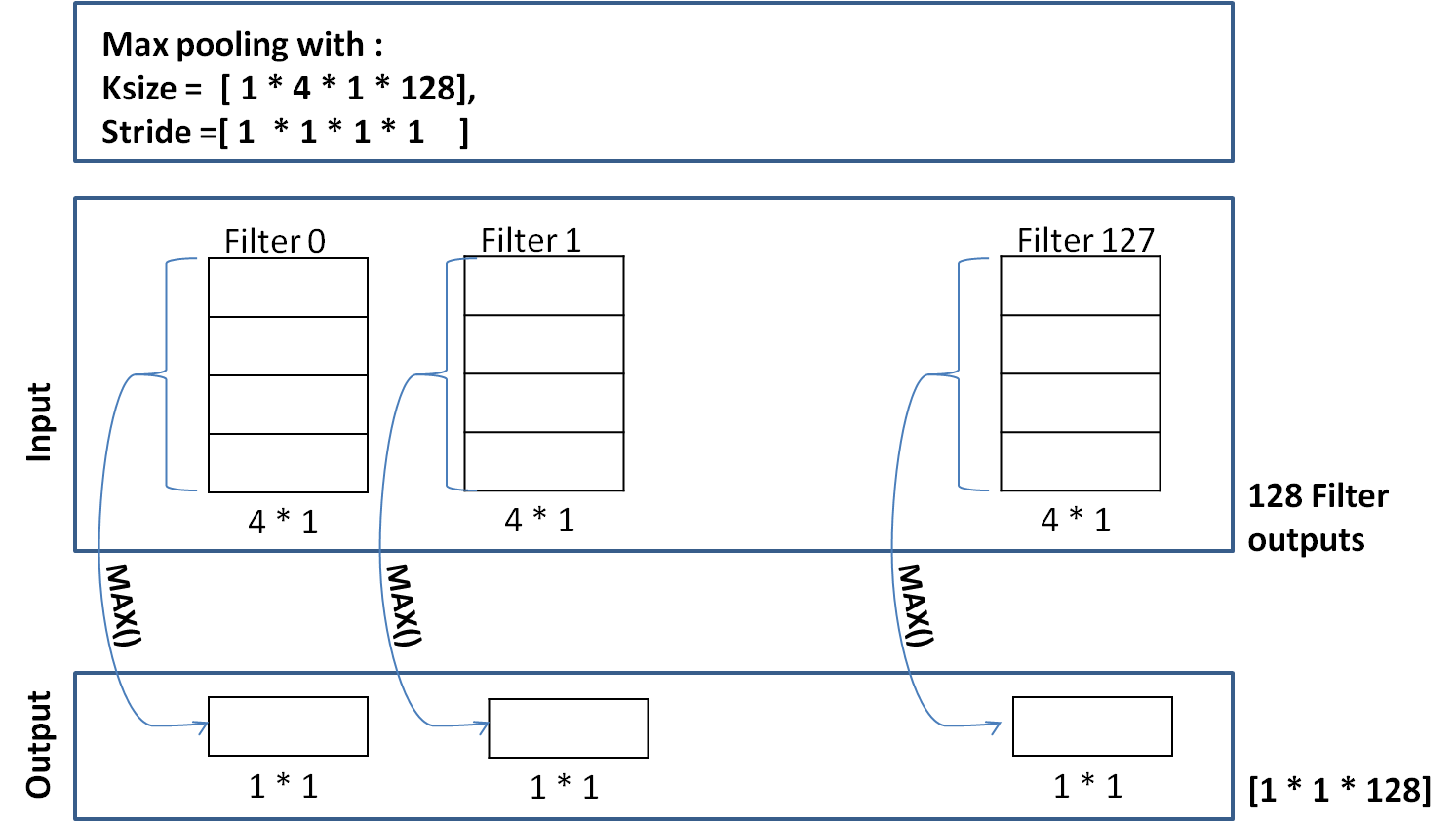
Therefore, we have max pooling output shape = [1 * 1 * 128] (128 - for each filter)

Now, suppose we change the ksize = [1 * 2 * 1 * 128], and stride = [1 * 1 * 1 * 1], we get output of shape [3 * 1] for each of 128 filters as shown below:

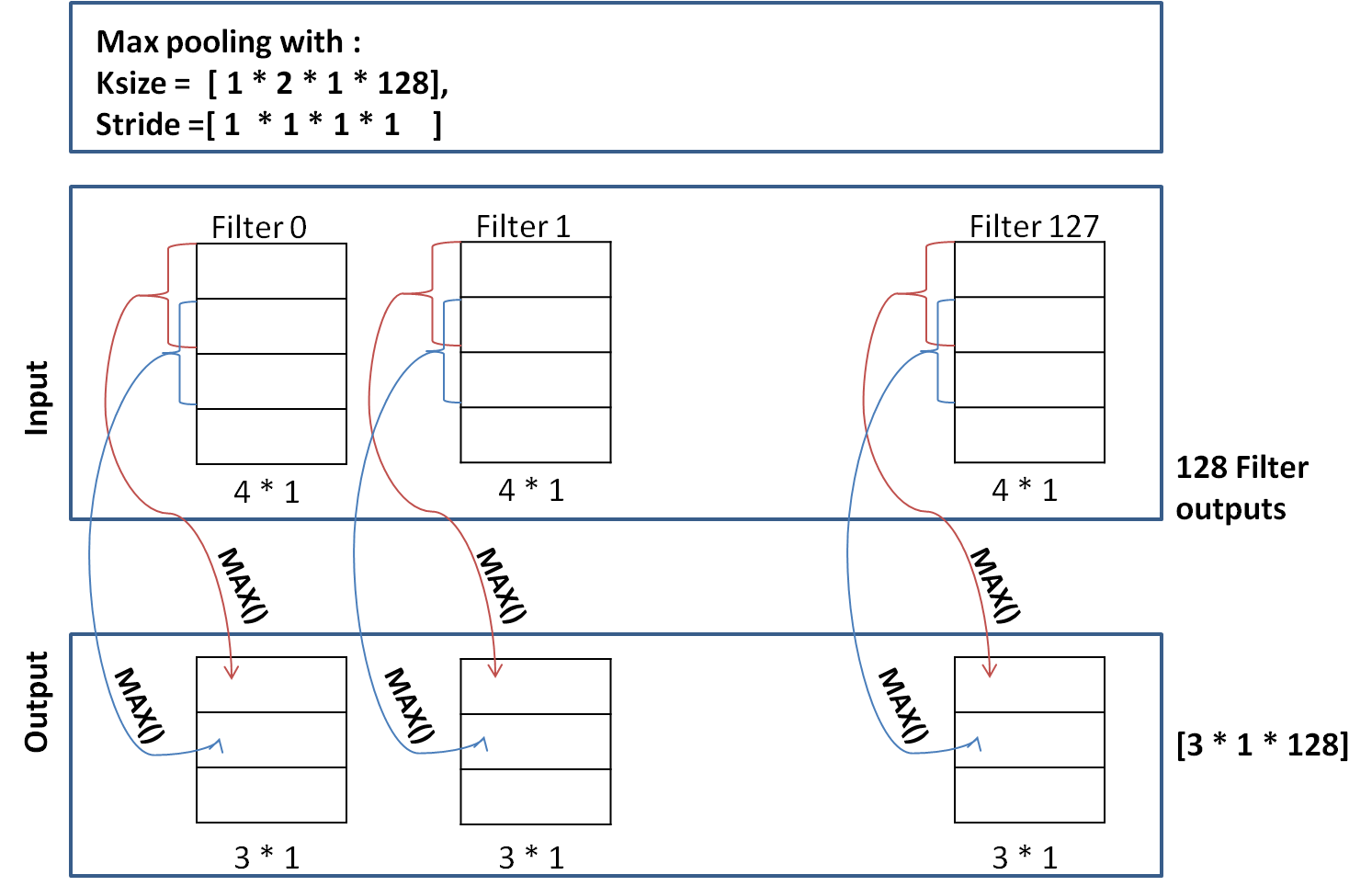
In our text classification problem filter moves only in one direction, therefore, size = 3 * 1. It it had moved along horizontal direction also (as in images), the shape of output would have been (3 * a) where a > 1

Merging the output of max pooling layer for each filter size(3, 4, 5).

Corresponding code statement:

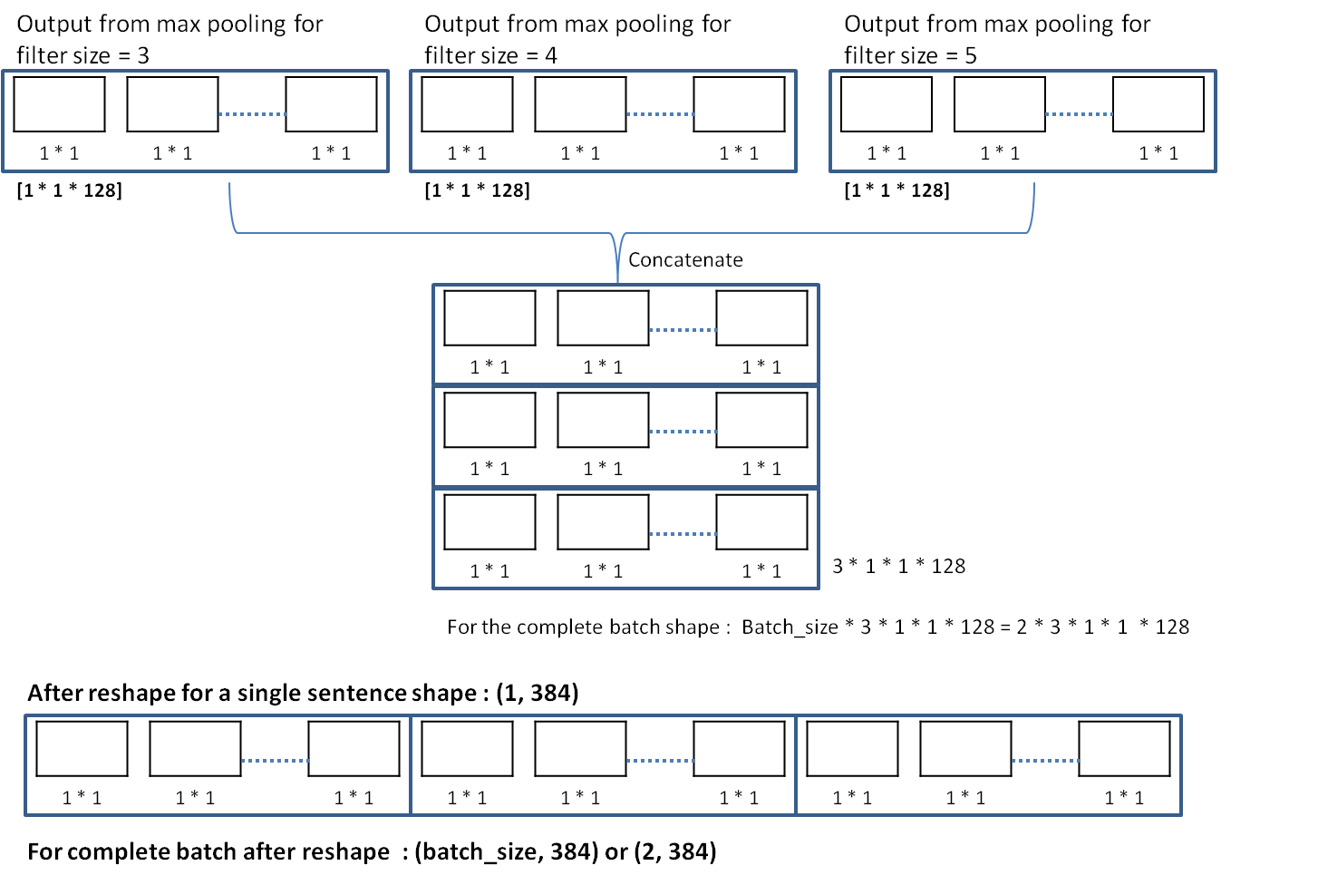
self.h_pool = tf.concat(3, pooled_outputs)

Now, for the current example we have 3 different filter size (3,4,5). For each filter size we get a tensor of shape [1 * 1 * 128]. These tensors are concatenated. So, we have 3 tensors of shape [1 * 1 * 128] to get a tensor of shape [3 * 1 * 1 * 128]. Since, the same is done for each sentence in the batch, shape of the tensor becomes [batch_size * 3 * 1 * 1 * 128] = [2 * 3 * 1 * 1 * 128] as shown below

Next, in the code,

 self.h_pool_flat = tf.reshape(self.h_pool, [-1, num_filters_total])

a reshape is performed to get a tensor of shape [batch_size, (3* 128)] = [batch_size , 384] = [2 * 384]. This means, now for each sentence we have a fiter output in a row as shown above.

Dropout Layer

Corresponding code statement

self.h_drop = tf.nn.dropout(self.h_pool_flat, self.dropout_keep_prob)

In this layer simply dropout is applied. Input and output shapes remain the same.

• Input shape : [batch_size * 384] = [2 * 384]
• Output shape : [batch_size * 384] = [2 * 384]

Output Layer

Corresponding code statement

self.scores = tf.nn.xw_plus_b(self.h_drop, W, b, name="scores")

Configurable parameters of output layer

• Weight matrix (W) of shape [ total_num_filters * num_classes]
  where, total_num_filters = length([3, 4, 5]) * num_filters = 3 * 128 = 384,
  num_classes = 2, Therefore, shape of W = [384 * 2]
• Bias (b) of shape [num_classes] = [2] or
  b = [0.1, 0.1]

Input

Output of the previous dropout layer with shape [2 * 384]. So, the size of each input vector is 384.

Working

For each input vector (x) from the previous layer, xW + b is calculated,
where x is a row vector of [384] elements, W is [384 * 2].
So, for each sentence we get a vector of length 2 (num_classes),
and, for the batch of size batch_size, output shape is [batch_size * num_classes] = [2 * 2] as shown below